
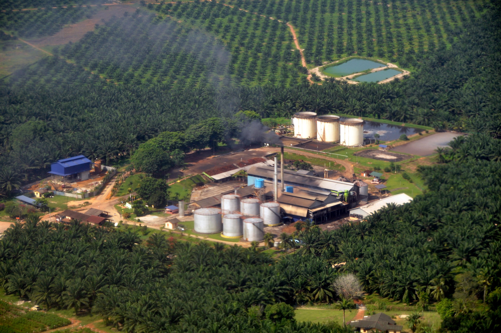
Of late, I have been appreciating how big the world is. We have been slicing its land surface into squares, hundreds of millions of them, and inquiring into each as to whether it boasts any notable concentration of cows. We’ve hit on a few surprises.
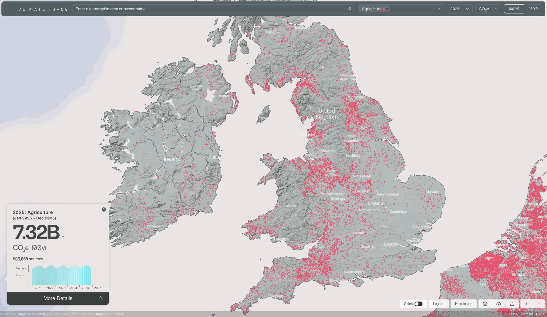
The work is for Climate TRACE, to improve greenhouse gas emissions tracking. Cows are prolific belchers of methane, and we are attempting to chart all of the world’s large beef feedlots and dairies. We use Earth Index, our AI tool to parse satellite imagery, with researchers at Saint Louis University’s (SLU’s) Remote Sensing Lab handling the modeling. To date we’ve covered half of the top 30 countries in cattle methane emissions, along with some others for various priorities, amounting to hundreds of thousands of facilities: A thousand farms and feedlots in Kansas. Two thousand farms and feedlots in Nebraska. Hundreds more across the US west. Nearly ten thousand dairies in Britain (Figure 1). Goshalas in India. Dairy colonies in Pakistan. And so on, to Japan to Argentina and Brazil, and back again. In many places, agricultural data only exist as aggregated statistics. Knowing locations of actual cows, we can analyze livestock and waste management practices and begin to discuss solutions.
Algorithmically, we are training lightweight classifiers on embeddings output by a geospatial foundation model (FM). For this project, we run the SSL4EO ViT-DINO on Sentinel-2 satellite image mosaics retrieved from Earth Engine. The classifiers have been small, fully-connected neural networks, although our recent benchmarking suggests these are likely over-fitting, and we should default to logistic regression.
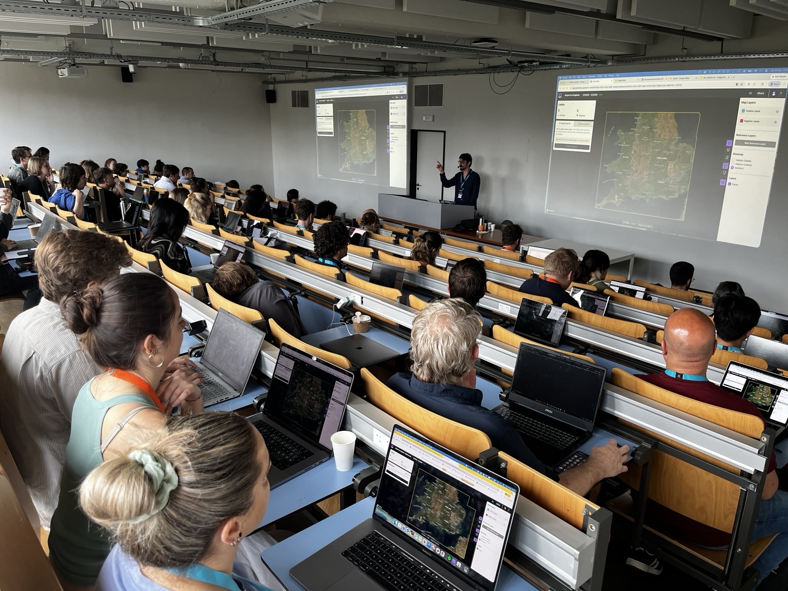
We build the training database on the fly. We gather seed examples from open data, including map search; we use Earth Index to run fast nearest-neighbor search of embedding vectors to gather further samples; we randomly sample negatives, which works well for sparse targets; and then we iterate training classifiers on successively larger datasets until we reach satisfactory performance. We validate using publicly available, high-resolution satellite basemaps, map labels, and occasionally, Street View. Up until now, classifier training has lived in a Jupyter notebook, but we are releasing it into the Earth Index web interface this spring.
I have written about this kind of modeling before, and I propose here to cover some things we’ve observed in scaling the process globally:
- Models extrapolated to new geographies tend to be useful but not, by themselves, good enough.
- For efficiency, consistency, and repeatability, we want to extend our models to cover continents.
- At critical points we have had to drawn on local linguistic and cultural knowledge.
Extrapolation and the BSI
In Nebraska, where I began exploring two years ago, the plains are studded with vast dusty feeding lots that can stretch miles on end. There are smaller family farms, where you might see a farmhouse, silos, stacked bales of hay, and a few backyard cow pens. In the west of the state, it’s drier, with more center-pivot irrigation and crumpled Rocky Mountain foothills. You start to see horse ranches. We confront sawmills, a composting center, a remote site with manure spread to dry in the sun – cow traces, without cows – and badlands along a river bottom detected for reasons I still don’t understand. These are the last holdouts tricking our models. The Earth reserves its right to its complexities.
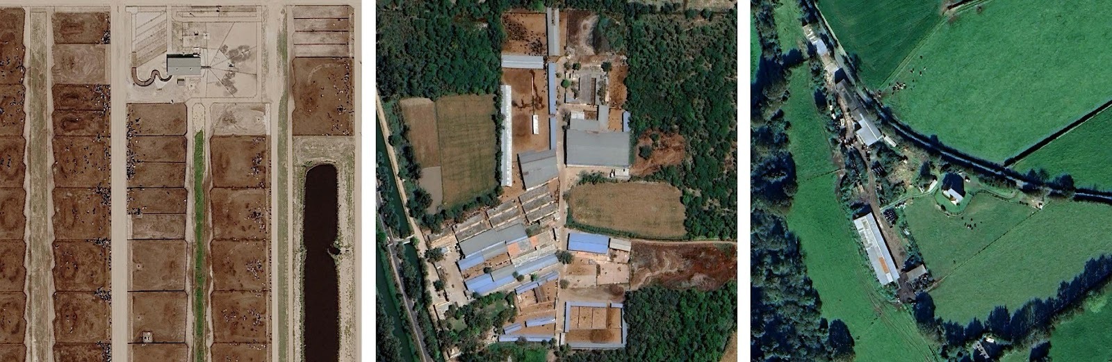
Even in a single U.S. state, there is so much terrain to account for, and Nebraska covers about half of one percent of the world’s arable and grazing lands. Each new region we survey twists the Nebraska pattern to its own ends, with different terrain, materials, and building and farming traditions (Figure 2).
We sometimes run an existing model on a neighboring state or country. A Nebraska model run on Kansas yields creditable outputs by itself. Much farther afield, we might see that half or fewer of the detections are valid. Certainly a Nebraska model is not going to suffice for India. This is clear on inspection, given that we’re targeting precisions, even for hard cases, near 90%. A transferred model can, however, serve as another way to find training samples for the new domain.
Earth Index shines in hopping from region to region, because of its quick modes for gathering training data, and because it takes relatively few samples, often only hundreds of positives, to train good classifiers when building on foundation model embeddings.
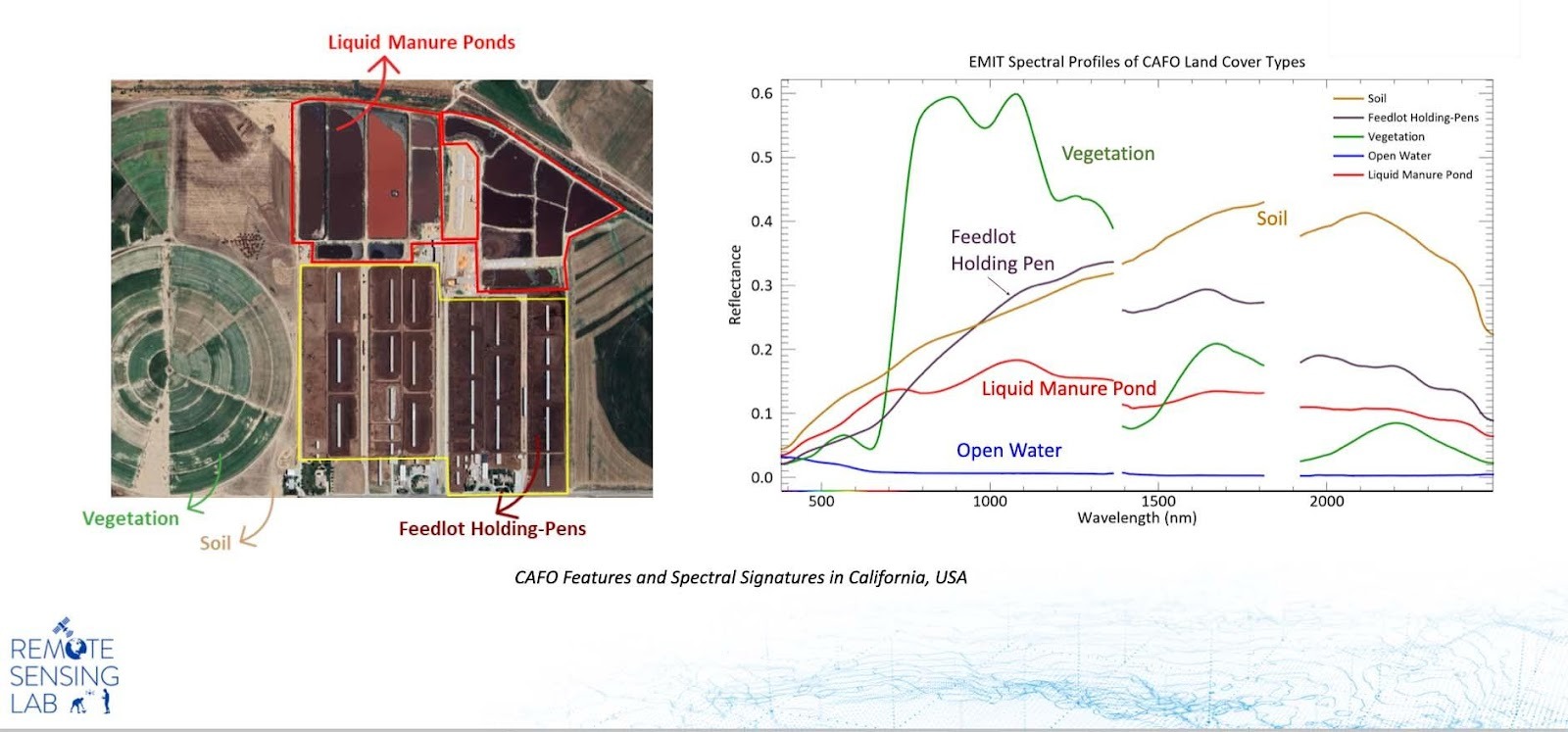
At first I wondered at how a model, trained on industrial feeding lots, could pick out a few cows in a desert village backyard. Mostly what they have in common is a deep-brown, manure-mixed, cow-trampled earth. It looks like any old dirt to the human eye, so our models have got to be cuing on a signature in its infrared spectrum to hone in on farms of such different forms.
This past year, our colleagues at SLU worked out the spectral separability of cow pens (the manure-mixed earth), and also liquid waste, using hyperspectral (Figure 3) and then Sentinel-2 satellite data. They just submitted the findings as a research paper and a proposal for a new remote sensing index, the Bovine Slurry Index, or the BSI.
You know what BSI really stands for.
The facts of your life creep up on you. Certainly I never dreamed of this when I was a kid. But at some point you have to acknowledge – and sorry, Mom, for saying it – that yes, my job is to monitor cow poop from space.
Duck DB and goshalas
My colleague Chris Ren showed me the Duck DB trick. In Nebraska, the embeddings database runs to 8 million 384-dimensional byte vectors, each with a point geometry attached. That’s about 3 GB on disk and a comparable burden on system memory when loaded into a Pandas GeoDataFrame. That’s still workable. To scale to bigger geographies, we now:
- Shift the embedding vectors into a DuckDB database. DuckDB is a small, pip-installed package to run SQL queries on local data files, from within Python.
- Continue loading point geometries into a GeoDataFrame, from a parquet file. Each point here represents the centroid of the square patch that has been embedded by the FM.
- Attach a unique string ID to each embedding vector and its corresponding centroid point, to link back and forth between.
For model training, we only need some thousands of embedding vectors loaded into memory, one for each labeled data point. (We snap data points to the nearest patch centroid.) And during model inference, it’s easy to read embedding vectors batch by batch from disk. With this reorganization, we have, for instance, fit embeddings for the whole South Asian subcontinent into a single dataset.
We have been experimenting with building models over larger regions. Scaling random negative sampling to cover all relevant terrain types is an easy, but essential step. It seems there are some economies to be had in positive labeling and plenty of expressiveness in the FM embeddings.
More to the point, we have by now a menagerie of models covering different states and countries, built at different times, and having undergone different degrees of validation. For consistency of the data, and to be able to run new assessments in the future, we will need to consolidate our findings through training a few geographically expansive and well-characterized models.
India has been an interesting study. India has the most cows of any country in the world. The animals are widely revered in Hindu tradition, and the country has no feedlots or beef industry to speak of. Initially, we didn’t know how to try to detect or otherwise characterize cattle that are spread around the country on small farms.
Ashutosh Pawar, a PhD student at the SLU Remote Sensing Lab, and originally from Maharashtra, drove a lot of our modeling in 2025 and the work on the BSI paper. He made sense of some fortuitous map labels near early model detections in north-central India. There are large concentrations of cows in India. They are called goshalas in Hindi (Figure 2), and they are shelters for stray animals. There are many thousands of them in the country.
Please no fart jokes
Animal agriculture is a major source of greenhouse gases, producing around a sixth of all emissions from human activities.¹ Among animals, beef herds are far and away the most polluting. Cattle facilities do range widely in their emissions,² which at least points to the possibility of targeted emissions reductions strategies. Ideas include limiting conversions of forest to grazing lands, improving degraded pasture, enclosing manure waste, and – we should say it – reducing the numbers of cows.
In facilities that have them, liquid manure slurry ponds tend to be the dominant source of methane emissions, as they afford ideal conditions for methanogenic archaea to digest waste. Globally, the biggest source of emissions from the cattle sector are the cows themselves. They release methane as they digest their food. It’s mostly cow burps, not cow farts, by which they release the potent greenhouse gas. Somewhere north of a billion bovines are burping in synchrony, the world over. This irreducibly fetid fact of cow life drives a search for biological interventions, including food additives, enzyme inhibitors, microbiome optimizations, grazing management, vaccines, and even direct methane capture from barn air or cow-wearables.
For the coming year, we are going to be improving model accuracy, training continental models, and running BSI over known facilities to detect manure waste ponds and improve emissions estimates.
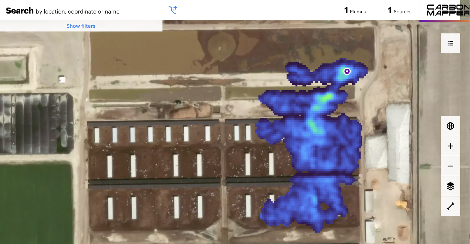
As of 2025, the Carbon Mapper and GHGSat satellites can detect methane emissions directly, at a fine enough resolution to measure fluxes from large single feedlots (Figure 4). As the data coverage and availability improves, it will be interesting to link up those measurements with ours.
1. Twine R. “Emissions from Animal Agriculture—16.5% Is the New Minimum Figure.” Sustain Sci Pract Policy 13:6276 (2021).
2. Poore J. and Nemecek T. “Reducing food’s environmental impacts through producers and consumers.” Science 360:6392, 987-992 (2018). doi: 10.1126/science.aaq0216.
Other articles

.png)
Engineering updates on sustainable AI at Earth Genome
Behind the scenes sustainability improvements on patch grid generation, STAC metadata, energy transparency, and DB optimization.


Launching Earth Index Deep Search for comprehensive planetary data
You can now train lightweight classifier models directly on the web
.png)