Earth Index Imagery V2

Today we’re excited to release the second version of our Sentinel 2 yearly composites with many major improvements in quality.

The quality improvements will cascade down into Earth Index leading to better search results and more impact on the ground. The process and efficiency improvements have reduced our pipeline costs by almost 65%, allowing us to move more quickly towards our goals of launching global coverage of Earth Index.

Of course none of this could have been possible without generous grants from the Patrick J. McGovern foundation, the Taylor Geospatial Institute and Amazon Web Services.

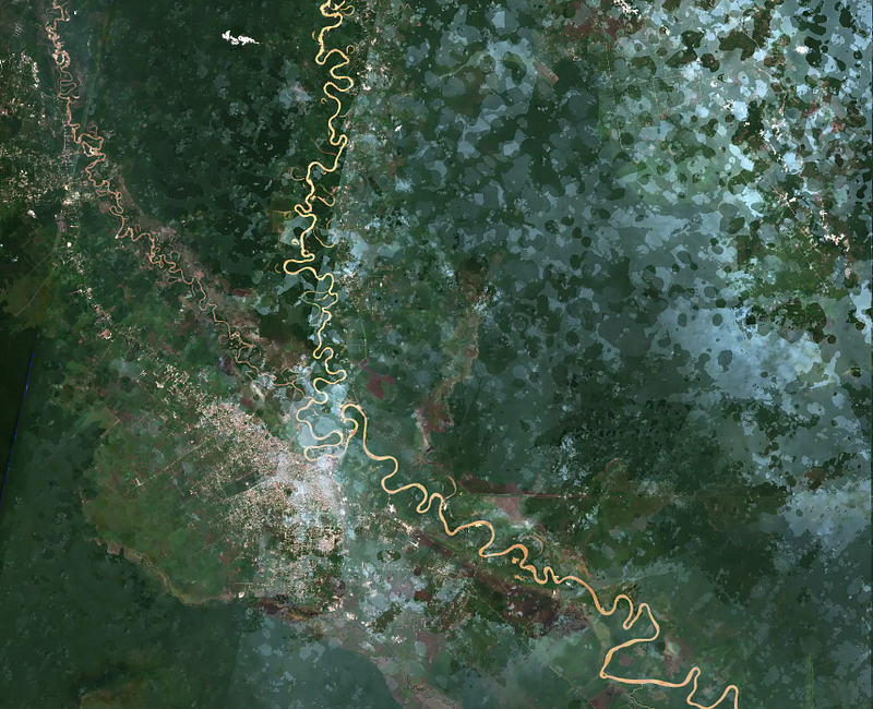
As before, full global coverage for 2022, 2023 and now 2024 will all be publicly available on Source.coop in the coming days. Coverage in select areas, notably the Amazon region, goes all the way back to 2018.

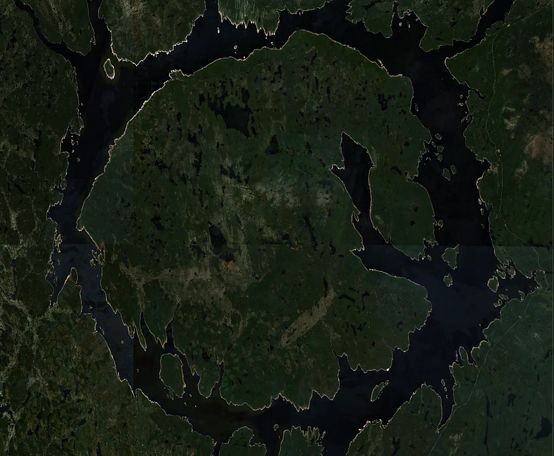
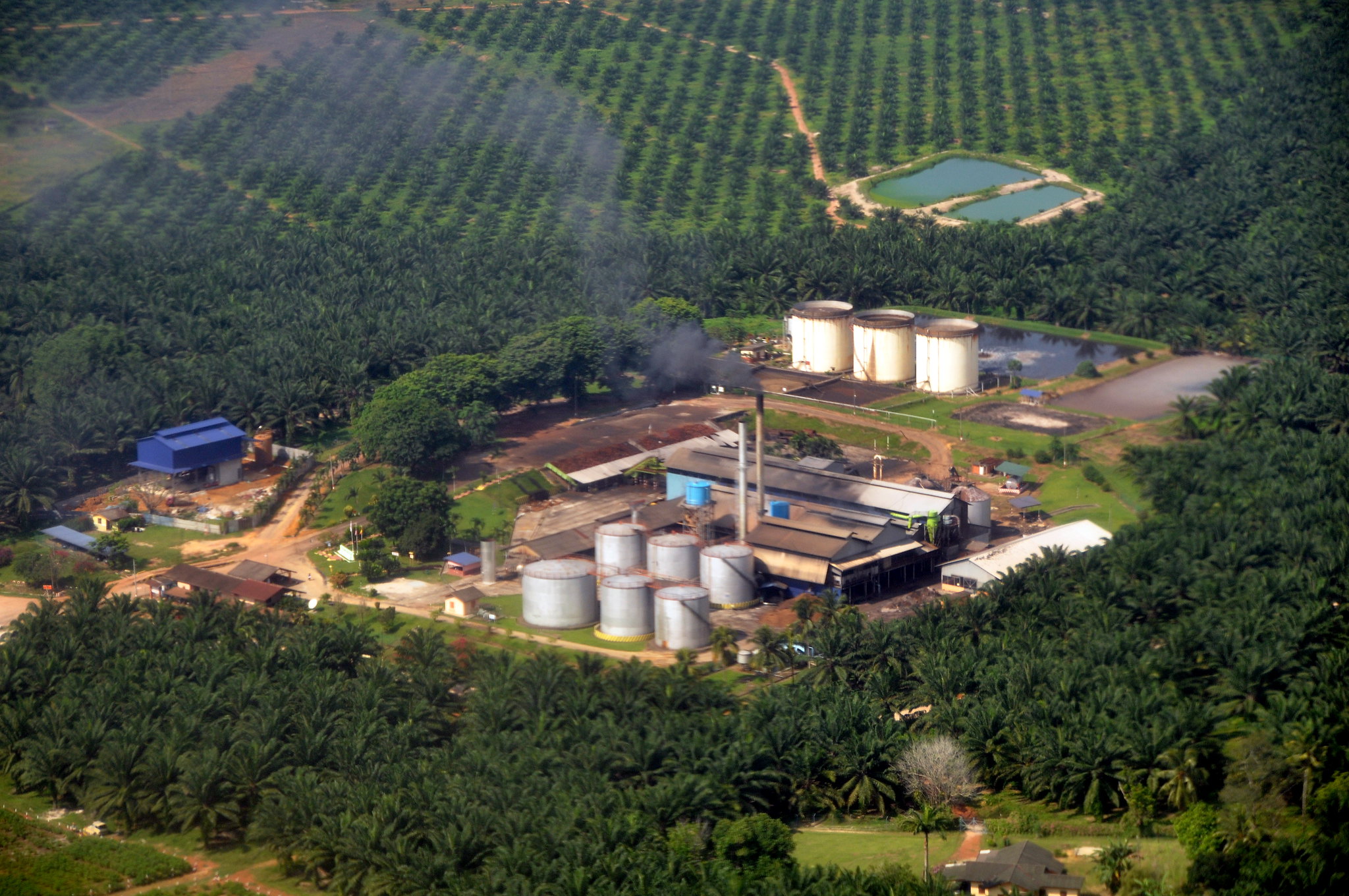
Before getting into the technical details of how we achieved the improvements, let’s peek at some imagery:

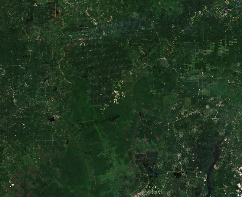
“If you are not embarrassed by the first version of your product, you’ve launched too late” — Reid Hoffman

While I wouldn’t quite say I’m embarrassed at the first version of our imagery, I will say that looking back at it now there was much room for improvement.

Our V1 imagery release was a major milestone for us, not only because it allowed us to achieve self-sufficiency in terms of cloud free imagery, but it was also our first major step to scale our pipelines (and hence our impact) to a global scale. It laid the foundation for a huge amount of growth and experimentation for technical and application challenges. Keeping in mind another of my favorite quips “Perfect is the enemy of good” it was extremely important for us to put a stake in the ground, launch it and move on to other challenges.

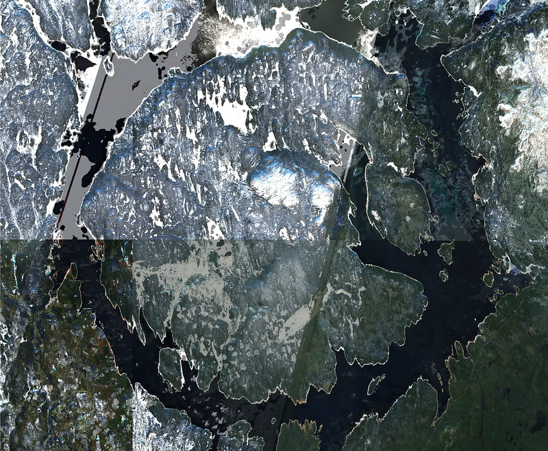
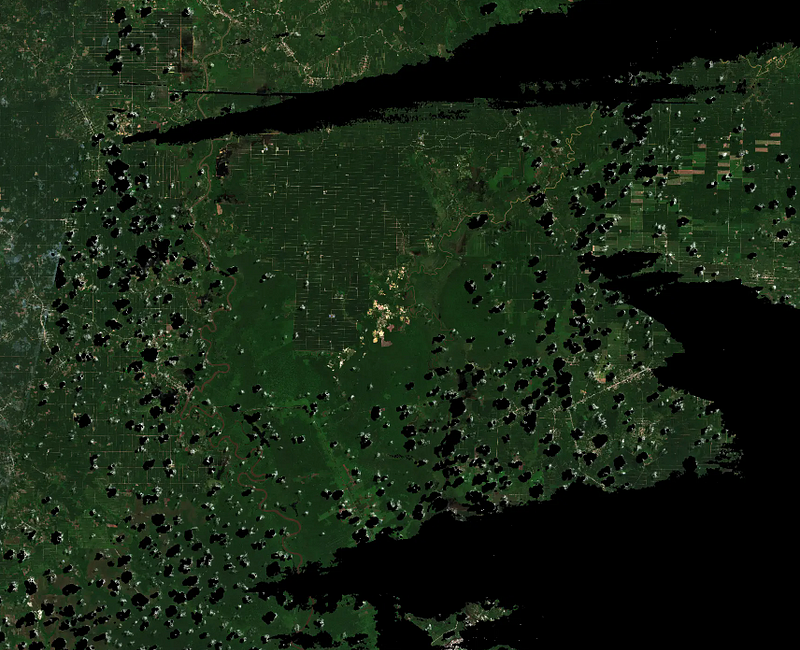
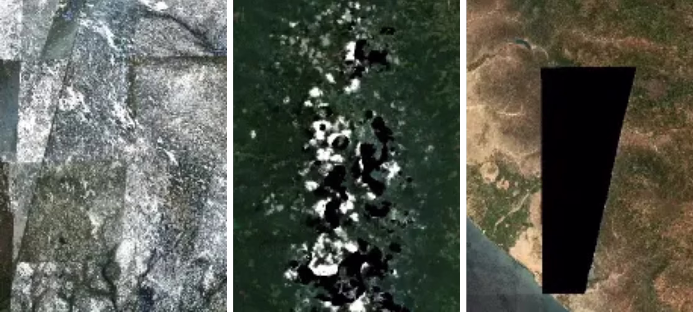
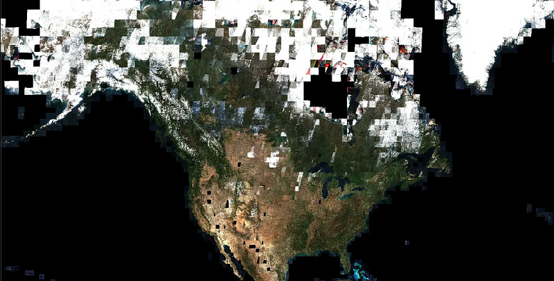
All that being said, we had several different types of issues we wanted to address in V2 as we prepared to process 2024–2025. In terms of quality we had large sections of no-data pixels, incomplete cloud masking and large swaths of snowy scenes.

We also wanted to improve the efficiency of the code and reduce resource requirements, runtime and overall cost.

Image Quality: When Metadata isn’t enough

It stands to reason that the best way to get a good quality mosaic is to use good quality source scenes. In V1 we used the EarthSearch STAC API with a BBOX query to find scenes matching the area we were processing (an MGRS grid cell) sorted by cloud cover. We would then evaluate the results to make sure to select full grid cells (and not neighboring cells) and use the top 16 to create a mosaic.

For V2 we started by looking at the other metadata fields in the STAC record that could give us hints as to the real quality of the scene. The metadata describes cloud cover, but also percentages of the image covered by snow, shadows, no data pixels, defective pixels and more.

Snow and ice are not necessarily bad — we want to include glaciers, for example, but not seasonal snow cover. Likewise, no data pixels (the culprit behind the black triangles above) are always present in some areas due to how orbits are split into MGRS tiles. If we only selected scenes with the lowest value of no-data pixels we would end up with mosaics that were missing the same small area in each scene. Even just selecting the lowest amount of cloud cover can be tricky in areas where clouds linger over the same mountain day after day.

While the easy answer seems to be to minimize negative metadata values, the reality isn’t as straightforward. Despite a low quality score, a scene might have just the area we were missing for the mosaic. And how many scenes should we use? The maximum would potentially waste compute but a smaller number producing a bad result would waste compute too. This is a real world example of a set cover problem, which is NP-Hard.

Rather than continuing to guess at how helpful an image might be for the mosaic, we decided to expand our scene selection process to download and preprocess SCLs (Scene Classification Layers) from candidate scenes. Our new scene selection is a 3 pass process that looks like this:

1st Pass: Search

Query STAC for records matching the MGRS tile we’re processing, order by cloud cover

2nd Pass: Preprocess and Evaluate

If the scene is the same MGRS ID, download and pre-process the SCL. Preprocessing consists of:

• Binary Dilation of pixels classified as cloud (effectively expanding cloud’s borders)
• Convert the various classification values into binary mask of good (1) and bad (0) pixels
• Caching the processed SCL

Add the candidate binary mask to an aggregation of previously selected candidate masks and evaluate the improvement. If adding the candidate results in a net improvement, keep it, otherwise discard.

Repeat until we reach a preconfigured maximum number of scenes or greater than 99.9% coverage with “good” pixels.

3rd Pass: Optimize

1. Re-rank the scenes selected in the second pass by the total percentage of good pixels in their preprocessed SCL.
2. Incrementally add them together as before, discarding any that are found to be redundant.

This reordering and implementation of the greedy algorithm can reduce the number of scenes by 30% or more — often significantly fewer scenes than V1 used.

Which Pixel is the right Pixel:

Now that we had our optimized list of candidate scenes, we then need to decide which parts (pixels) of which scenes to use for the final composite. Because the scenes are from different times across the year, it’s critical to figure out a good strategy to pick the pixel that is most representative for that spot on the earth over the course of the year.

Pixel selection is a hot topic here (we don’t get out much) so lots of experimentation ensued to see how different strategies would affect the output.

It seems clear that min and max aren’t appropriate for a yearly representative value, and mean was rejected as it wasn’t a “real” sensed value. After some trial and error we found that the 1st quartile value seemed to work quite well. It favored “darker” pixels that would avoid snow and prefer summer in both hemispheres.

Performance: Time is Money

These changes in scene and pixel selection methods gave us huge improvements in coverage and quality; however there were also significant code tweaks in processing that helped us achieve our cost and efficiency goals.

As with many things in the python ecosystem, there are about 100 ways to do anything. We undertook an evaluation of each step in the processing code and looked for suspicious slowdowns, needless to say we found many. This is not an exhaustive list, but just a few of my favorite lessons:

• GDAL is almost always faster and more performant than anything else. Take the time to learn the less well known parameters. We stand on the shoulders of giants (Frank, Even and others)
• There can be a big performance difference between seemingly similar Numpy functions. np.min/np.max is much quicker than np.median, which is much quicker than np.quartile
• Numpy dtypes matter, and not just for memory management — did you know np.nan is a float?!
• Dask/Xarray chunking works well — if you let it. It’s easy to create lots of independent arrays and combine them later. But doing so prevents Dask from properly estimating memory usage and chunking automatically. Better to sensibly chunk and OOM less
• Your local machine’s SWAP makes you think your code is memory efficient. It is not.

This deep review alone dropped our processing time by an order of magnitude.

Arm is worth it

As one of the last remaining people with an Intel Mac (or so it seems), I was hesitant to port any of our workloads to Arm. But trying to find the optimal instances to run I kept coming back to the low cost of the various AWS Graviton families. Trying them was uneventful, in a good way. My fears of “raspberry pi”-eqsue performance were unfounded and they seemed to be the equivalent of a normal x86–64 instance and a fraction of the cost. Sold.

Look for more exciting news about the next stages of Earth Index and global availability in the coming weeks!!

‍